


Metrics Available for Both Blocking Mesh and Body Mesh
Jacobian Ratio
The Jacobian Ratio metric compares the shape of a given element to that of an ideal element. If an element has a poor Jacobian ratio, the element may not map well from element space to real space, thereby making computations based on the element shape less reliable. The ideal shape of a hexahedron has all flat sides and 90 degree angles.
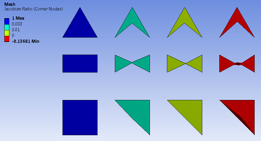
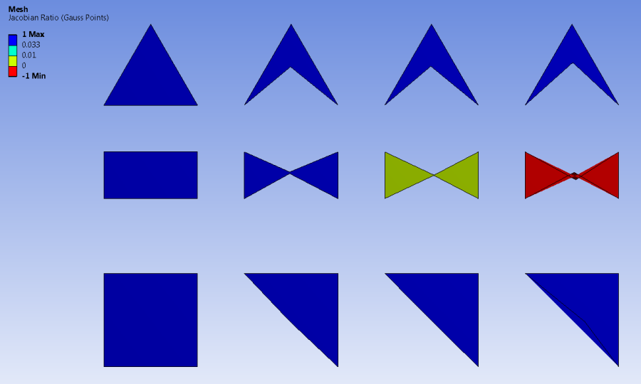
There are two ways to calculate the Jacobian Ratio, either based on Corner Nodes (nodal points) or based on Gauss Points (integration points). The corner node calculation is more restrictive while the Gauss points calculation is less restrictive. In either case, the value is bounded by -1 (worst) and 1 (best). An element with Jacobian ratio <= 0 should be avoided.
An element's Jacobian ratio is computed by the following steps and using all available nodes for the element:
At each sampling location listed in the table below, the determinant of the Jacobian matrix is computed and called RJ. At a given point, RJ represents the magnitude of the mapping function between the element's natural coordinates and real space. In an ideally-shaped element, RJ is relatively constant over the element, and does not change sign.
Element Shape RJ Sampling Locations for corner nodes calculation RJ Sampling Locations for corner nodes calculation 8-node bricks Corner nodes Choose the optimal number of Gauss quadature points for integration 20-node bricks All nodes and centroid Eight Gauss quadrature points The Jacobian ratio of the element is the ratio of the minimum to the maximum sampled value of RJ.
The Jacobian ratio of an ideal hexahedral element is 1, indicating (a) its opposing faces are all parallel to each other, and (b) each midside node, if any, is positioned at the average of the corresponding corner node locations. As a corner node moves near the center, the Jacobian ratio worsens. If the node is moved significantly, the Jacobian ratio will become negative and the element is invalid.
The figure below illustrates the Jacobian ratio metric by color for various element shapes.
Aspect Ratio
-
When High Fidelity is enabled, the Aspect Ratio metric is calculated using the ratio of the lengths of sides. The details vary depending on the type of surface element (face).
Aspect Ratio Calculation for Triangles
The aspect ratio for a triangle is computed in the following manner, using only the corner nodes of the element.
For each node (I, J, and K in the following image), a line is constructed from that node of the element to the midpoint of the opposite edge, and another through the midpoints of the other 2 edges. In general, these lines are not perpendicular to each other or to any of the element edges.
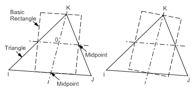
Rectangles are constructed centered about each of the 2 lines, with two edges parallel to one of the lines, and all edges passing through the element edge midpoints and the triangle apex.
These constructions are repeated using each of the other 2 corners as the apex.
The Aspect Ratio of the triangle is the ratio of the longer side to the shorter side of whichever of the 6 rectangles is most stretched, divided by the square root of 3.
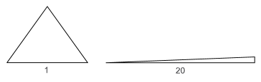
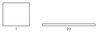
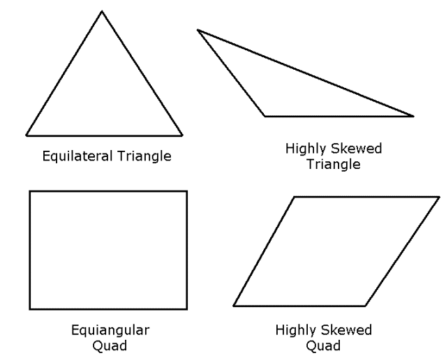
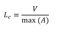
The best possible triangle aspect ratio occurs for an equilateral triangle and is 1. A comparison between an equilateral triangle and a triangle having an aspect ratio of 20 is shown below.
Aspect Ratio Calculation for Quadrilaterals
The aspect ratio for a quadrilateral is computed by the following steps, using only the corner nodes of the element.
- If the element is not flat, the nodes (I, J, K, and L in the following image) are projected onto a plane passing through the average of the corner locations and perpendicular to the average of the corner normals. The remaining steps are performed on these projected locations.
- Two lines are constructed that bisect the opposing pairs of
element edges and which meet at the element center. In general,
these lines are not perpendicular to each other or to any of the
element edges.
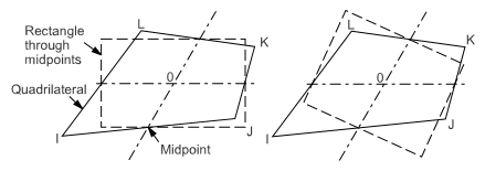
- Rectangles are constructed centered about each of the 2 lines, with two edges parallel to one of the lines, and with all edges passing through the element edge midpoints.
- The Aspect Ratio of the quadrilateral is the ratio of a longer side to a shorter side of whichever rectangle is most stretched.
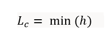
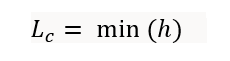
The best possible quadrilateral aspect ratio occurs for a flat square and is one. A comparison between a square and a quadrilateral having an aspect ratio of 20 is shown below.
Aspect Ratio for Hexahedra
The Aspect Ratio metric for hexahedral elements is defined as the size of the minimum element edge divided by the size of the maximum element edge. The values are scaled and the default range of values is 1-20, such that an Aspect ratio of 1 indicates a regular element.
-
When High Fidelity is disabled, the Aspect Ratio metric is calculated for different element types as follows:
Aspect Ratio for Quadrilaterals/Pyramids
The aspect ratio is the Determinant, which is the ratio of the smallest determinant of the Jacobian matrix divided by the largest determinant of the Jacobian matrix, where each determinant is computed at each node of the element. A value of 1 would indicate a perfectly regular mesh element, 0 would indicate an element degenerate in one or more edges, and negative values would indicate inverted elements.
Aspect Ratio for Prisms
The quality is calculated as the minimum of the Determinant and Warpage. The Determinant is the ratio of the smallest determinant of the Jacobian matrix divided by the largest determinant of the Jacobian matrix, where each determinant is computed at each node of the element. Warpage is normalized to a factor between 0 to 1, where 90 degrees is 0, and 0 degrees is 1.
Aspect Ratio for Hexahedra
The quality is a weighted diagnostic between Determinant (between -1 and 1), Max Orthogls (normalized between -1 and 1; if deviation from orthogonality is greater than 90 degrees, then the normalized value will be smaller than 0) and Max Warpgls (normalized between 0 and 1; warpage of 0 degrees is 1, warpage of 180 degrees is 0). The minimum of the 3 normalized diagnostics will be used.
The Determinant is the ratio of the smallest determinant of the Jacobian matrix divided by the largest determinant of the Jacobian matrix, where each determinant is computed at each node of the element.
The Max Orthogls calculates the maximum deviation of the internal angles of the elements from 90 degrees. For hexahedra, angles between 180 and 360 degrees are also considered (deviation up to 270 degrees).
To determine the warp of a quadrilateral face, the angles between the triangles connected at the 2 diagonals of the quad will be calculated and the maximum will be used. The maximum warp of the hexahedral element is the maximum warp of its quad faces.
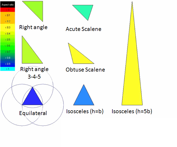
Aspect Ratio for Triangles
The ratio between the area of triangle and the maximum edge length for each element is calculated. The values are scaled, so that an aspect ratio of 1 corresponds to a perfectly regular element, while an aspect ratio of 0 indicates that the element has zero area.
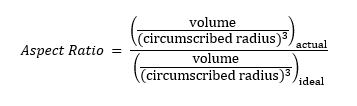
Aspect Ratio for Tetrahedra
The ratio between the volume of the element and the radius of its circumscribed sphere power three is calculated. The values are scaled, so that an aspect ratio of 1 corresponds to a perfectly regular element, while an aspect ratio of 0 indicates that the element has zero volume.
Element Quality
The Element Quality metric provides a composite quality value that ranges between 0 and 1. This metric is proportional to the ratio of the area to the sum of the square of the edge lengths for quad/tri surface elements, or the ratio of the volume to the square root of the cube of the sum of the square of the edge lengths for volume elements. A value of 1 indicates a perfect cube or square while a value of 0 indicates that the element has a zero or negative volume.
This can also be expressed as follows:
For quad/tri surface elements,  , where c represents a constant which depends on the element
type.
, where c represents a constant which depends on the element
type.
For brick volume elements,  , where c represents a constant which depends on the element
type.
, where c represents a constant which depends on the element
type.
The following table lists the value of C for each type of element:
| Element | Value of C |
| Triangle | 6.92820323 |
| Quadrangle | 4.0 |
| Tetrahedron | 124.70765802 |
| Hexahedron | 41.56921938 |
| Wedge (prism) | 62.35382905 |
| Pyramid | 96 |
Orthogonal Quality
The Orthogonal Quality metric is computed using the face (edge) normal vectors and vectors between centroids of adjacent cells (faces, edges). The range for orthogonal quality is 0 - 1, where a value of 0 is worst and a value of 1 is best.
Orthogonal quality is the default metric when the Physics Type is set to Fluid Dynamics.
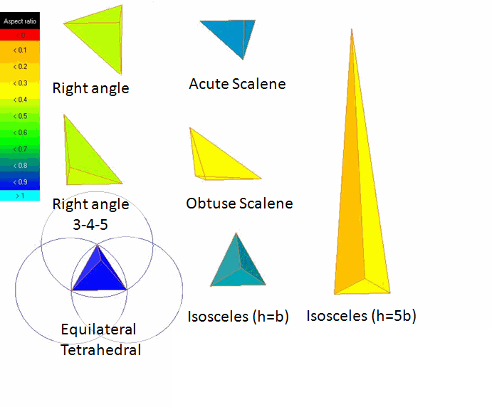
The Orthogonal Quality for 3D cells is computed using the face normal vector
( ) for each face, the vector from the cell centroid to the
centroid of each of the adjacent cells (
) for each face, the vector from the cell centroid to the
centroid of each of the adjacent cells ( ), and the vector from the cell centroid to the centroid each
of the faces (
), and the vector from the cell centroid to the centroid each
of the faces ( ). The image below illustrates the vectors used to determine
the orthogonal quality for a cell.
). The image below illustrates the vectors used to determine
the orthogonal quality for a cell.
For each face, the cosines of the angle between  and
and  , and between
  and
and  , are calculated. The smallest calculated cosine value is the
orthogonality of the cell. Finally, Orthogonal Quality
depends on cell type:
, are calculated. The smallest calculated cosine value is the
orthogonality of the cell. Finally, Orthogonal Quality
depends on cell type:
- For tetrahedral, prism, and pyramid cells, the Orthogonal Quality is the minimum of the orthogonality and (1 - cell skewness).
- For hexahedral cells, the Orthogonal Quality is the same as the orthogonality.
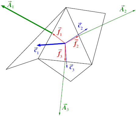
In a similar way, Orthogonal Quality for 2D faces is computed as the smallest
cosine of the angle between the edge normal vector,  for each edge and the vector from the face centroid to the
centroid of each edge,
for each edge and the vector from the face centroid to the
centroid of each edge,  . The image below illustrates the vectors used to determine
the orthogonal quality for a face.
. The image below illustrates the vectors used to determine
the orthogonal quality for a face.
- When the cell is located on the boundary, the vector
 across the boundary face is ignored during the quality
computation.
across the boundary face is ignored during the quality
computation. - When the cell is separated from the adjacent cell by an internal wall (a
baffle), the vector
 across the internal boundary face is ignored during the
quality computation.
across the internal boundary face is ignored during the
quality computation. - When the adjacent cells share a parent-child relation, the vector
 is the vector from the cell centroid to the centroid of
the child face while the vector
is the vector from the cell centroid to the centroid of
the child face while the vector  is the vector from the cell centroid to the centroid of
the adjacent child cell sharing the child face.
is the vector from the cell centroid to the centroid of
the adjacent child cell sharing the child face.
Inverse Orthogonal Quality = 1 - Orthogonal Quality
The orthogonal quality values may not correspond exactly with the inverse orthogonal quality values in Ansys Fluent because the computation depends on boundary conditions on internal surfaces (WALL vs. INTERIOR/FAN/RADIATOR/POROUS-JUMP). Ansys Fluent may return different results which reflect the modified mesh topology on which CFD simulations are performed.
Skewness
The Skewness metric is one of the primary quality measures for a mesh. Skewness determines how close to ideal (equilateral or equiangular) a face or cell is. The image below compares highly skewed faces to ideal faces.
The following table lists the range of skewness values and the corresponding cell quality.
| Value of Skewness | Cell Quality |
|---|---|
| 1 | degenerate |
| 0.9 — <1 | bad (sliver) |
| 0.75 — 0.9 | poor |
| 0.5 — 0.75 | fair |
| 0.25 — 0.5 | good |
| >0 — 0.25 | excellent |
| 0 | equilateral |
According to the definition of skewness, a value of 0 indicates an equilateral cell (best) and a value of 1 indicates a completely degenerate cell (worst). Degenerate cells and slivers are characterized by nodes that are coplanar or nearly coplanar (colinear in 2D).
Highly skewed faces and cells are unacceptable because the equations being solved assume that the cells are relatively equilateral/equiangular.
Two methods for measuring skewness are:
- Based on the equilateral volume (applies only to triangles and tetrahedra).
- Based on the deviation from a normalized equilateral angle. This method applies to all cell and face shapes, including pyramids and prisms.
Equilateral-Volume-Based Skewness
In the equilateral volume deviation method, skewness is defined as
 , where the optimal cell size is the size of an equilateral
cell with the same circumradius.
, where the optimal cell size is the size of an equilateral
cell with the same circumradius.
Quality meshes have a skewness value of approximately 0.1 for 2D and 0.4 for 3D. The table above provides a general guide to the relationship between cell skewness and quality.
In 2D, all cells should be good or better. The presence of cells that are fair or worse indicates poor boundary node placement. You should try to improve your boundary mesh as much as possible, because the quality of the overall mesh can be no better than that of the boundary mesh.
In 3D, most cells should be good or better, but a small percentage will generally be in the fair range and there are usually even a few poor cells.
Normalized Equiangular Skewness
In the normalized angle deviation method, skewness is defined (in general) as
 , where
θ max = largest angle in the face or cell
θmin = smallest angle in the face or cell
θe = angle for an equiangular face/cell (60 for a triangle, 90 for a square)
For a pyramid, the cell skewness will be the maximum skewness computed for any face. An ideal pyramid (skewness = 0) is one in which the 4 triangular faces are equilateral (and equiangular) and the quadrilateral base face is a square. The guidelines in the table above apply to the normalized equiangular skewness as well.
Characteristic Length
Characteristic length (also called characteristic dimension) is used to compute the time step that satisfies the Courant-Friedrichs-Lewy (CFL) condition for a given analysis setup. The CFL condition is of interest mostly in explicit dynamics and computational fluid dynamics analyses. It governs the maximum time step for which a solution will be stable.
The characteristic length is defined based on the element type.
For hexahedral elements:
where:
Lc = characteristic length of the hex element
V = volume of the hex element
A = area of the element face
For tetrahedral elements:
where:
Lc = characteristic length of the tet element
h = height of the tet element from a node to its opposite face.
For pyramid elements: (5-node solid element)
where:
Lc = characteristic length of the pyramid element
h = height of the apex node to the base of the pyramid. Here, the base quad face can be divided into 4 different triangles, the minimum height to these 4 triangles is used.
For Shell quad elements:
where:
Lc = characteristic length of the quad element
A = element area
L = element edge length
D = diagonal of the quad element
For Shell tri elements:
where:
Lc = characteristic length of the tri element
A = element area
L = element edge length